METHOD OVERVIEW
2.1 Introduction
Most ERP experiments demand some sort of task from the subject but the task is the same on each trial. The resultant potential is assured to be one which occurs with each trial but require averaging to improve the signal to noise ratio. In these experiments we expect the brain to change during repeated performance of the task so that the potential at the start of the experiment is expected to be different from that at the end. Once the experiment has been done it can not be repeated in the same subject as he or she is no longer naive to the task.
A further complication was that learning was accomplished by forming and testing internal hypotheses. Developing the subjects revealed a wide variety of learning hypotheses which were all wrong (except in one instance) but many hypotheses allowed that subjects to perform adequately and be classed as learners.
Unlike most ERP studies we had to monitor the performance of subjects throughout to assess their learning ability at the task.
Fortunately about half the subjects learned and half did not.
2.2 Subjects
Ninety-nine young adult volunteers participated in different experiments during the study. They were free from any significant diseases, such as brain damage, and all the diseases of the nervous system and all had normal or corrected to normal vision. They were given a full verbal explanation of the recording procedure, taken from the research information sheet (appendix 5.1.), and they were given a brief tour in the laboratory. A general questionnaire (Appendix 5.2.), fulfilled from each participant about his/her personal details, and state of health. Written consent was obtained from the subjects who were interested to continue.
Ethical approval was obtained from the Local Ethical Committee for the ERP experiments (041/99)
2.3. Subject’s handedness:
The subjects were questioned about:
All subjects are right handed as indicated in a chart of Edinburgh Handedness inventory (Oldfield. 1971) Appendix 5.3.
2.4. Task
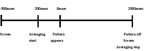
Subjects viewed 200 images of two types and had to recognise them as type A or type B indicating their decision by pressing one of two buttons within two seconds. These two hundred categorisation trials were broken into quartiles (four groups of 50 trials) for purposes of statistical analysis. All the images are individually different but belonged to type A or B. each image (stimulus) was presented for Duration of 2000msec, and was followed by a 500msec interval during which the screen was blank.
2.5. Images
The images were computer generated in black and white, with equal numbers of black and white pixels, so there were no brightness changes. Their properties were as follows.
|
Elements |
Pattern A (Fig. 8). |
Pattern B (Fig. 7) |
|
Element I |
50 % |
50 % |
|
Element II |
50 % |
50 % |
|
Element III |
37.5 % |
12.5 % |
|
Element IV |
12.5 % |
37.5 % |
Table (2.1.) the distribution of the four elements in bot patterns A and B.
![]()
![]()


(a) (b)
Figure (2.1.) shows the two-task images (a) type 1 or type A, and (b) type 2 or type B
2.6. Recording montage
The locations for these electrodes include all the standard international 10-20 system location (Jasper, 1958). In this system, the recording site of each electrode is specified in terms of its proximity to particular region of the brain and the subscript Z for midline: frontal (Fz), central (Cz), parietal (Pz) and occipital (0z). Odd number for the left side and even numbers for the right side of the location in the lateral plane over frontal (F3, F4) and (F7, F8), temporal (T3, T4), parietal (P3, P4) and occipital (01, 02) sites. Picton et al. (1978) have suggested an elaboration of the 10-20 system to include the specification of sites which lie between the standard locations (mostly halfway), and which are more suitable for evoked potential recording.
Additional scalp derived sites along with some electrodes fixed to the cap in appropriate positions, these sites were employed in a pattern previously used in ERPs language studies (Holcomb, and McPherson 1994; Holcomb, 1993; Holcomb & Neville, 1991). These include the following:
Left and right temproparietal TPL & TPR which were over the Wernicke’s area and its right hemisphere homologue (WL - WR 30 % of intra-aural distance. Lateral to point 13% of the nasion-inion distance posterior to CZ.
Left and right anterior temporal ATL & ATR 50% of the distance between T3/T4 and F7/F8
Three midline sites. FCZ 50% of the distance between FZ and CZ, OZ 10% of the inion-nasion distance and POZ 50% of the distance between PZ and OZ, These electrodes were concentrated over the areas of interest, the frontal, the parietal, and the temporal (Figure 2.2.)
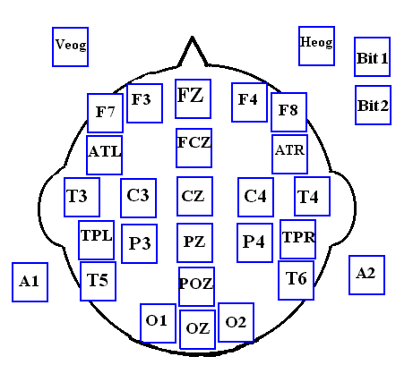
Figure (2.2.) shows my study electrodes and cap electrodes scalp montage position for placement of ERP recording. The abbreviation stand for A= Auricle, C= Central, F= Frontal, Fp = Frontal-pole, O= Occipital, P= Parietal, and T= Temporal. The odd numbers represent the left hand side electrodes, the evens numbers represent the right hand side electrodes, and letter Z represent the central line.
2.7. Electrodes
A few general rules made the studies easy to perform and greatly reduced the number of examiner errors. The electrode site on the patient’s skin is cleaned and free of oil, grease, and soil. The site of the electrode should be cleaned and abraded, as necessary, to reduce impedance at the electrode/skin interface.
All the recording points are measured in correct way and markedly clearly with visible ink. All electrodes are electrically tested for broken wires or defective contact points, if defecte repair or replace the electrode.
The electrode must be washed after each application; sometimes possible to draw blood during the scarifying process, and the risks of cross-infection must always be considered.
The event related potentials (ERPs) recorded by electroencephalography (EEG) electrodes of the tin disc or "stick on" type which consists of cupped disc, about one centimetre in diameter, a conducting medium (electrolyte), commonly isotonic (gel solution), is needed to act as a transmission bridge between skin and electrode. The skin/Electrolyte/Electrode interface, forms the first and in many ways the most vital link for faithful recording of scalp potentials. Neglect in the care of the electrodes, and poor application, leads to the most common recording problems. The capacitative and resistance depend on such factors as the kind of electrode metal, the nature, concentration, and temperature of electrolyte, and the frequency and density of the current passed.
The electrode was attached before to the scalp by the collodion adhesive applied round the rim of the electrode, the adhesive being dried by a steam of air from an air gun, or alternatively, bentonito electrode past is available used to hold the electrodes to the scalp and also offer a minor degree of adheasiveness, others prefer to place a small square gauze over the electrode disc and cove this with collodion, having beforehand vigorously rubbed the area underlying the electrode with a swab impregnate with saline, gel or wiped the skin with alcohol swab or a specially formulated compound.
A more recent development is the used blenderm or transport tape, approximately 2.5 centimetre. being taped over the electrode and hair holding the electrode firmly in place of normal length of a ERPs recording.
The electrode has a hole in the cupped part through which a needle can be inserted, inserting electrode gel into the cup; the electrode may be removed after use by pulling off the blenderm tape or by dissolving the collodion with acetone. This is an inflammable aliphatic solvent and care must be taken, so it must be administered sparingly to minimise the amount of fumes, which can irritate the eyes and the throat of both the subject and the recordist. It is strongly advisable to use vinyl shoulder cape on the patient to protect clothing. The eyes must be protected with eye pads when removing the frontal area electrodes.
Electrodes have a finite life (between 60 to 100 recording) usually failing due to breakdown at the joint between the electrode and lead.
2.8. Sterilisation
To avoid the possibilities of cross infection through the use of unsterilized electrodes by the most transmittable diseases have been particularly highlighted: AIDS, hepatitis B, and Creutzfeldt-jacob disease. All have been shown experimentally to be transmitted by cross -contact of blood host and recipient.
Guidelines have now been published for the laboratory and recording staff on how to handle the subjects and on routine and special procedure for sterilising electrodes and other equipment. For during and after use, the recording head stick-on electrodes are treated by ten minutes immersion in 0.1 % hypochlorite. Stick-on electrodes with autoclaved leads can now be readily purchased. Electrodes used for patient known to have, Creutzfeldt-jacob disease, should not be used again, and should be destroyed by incineration.
If secretion from infected patient (coughing, sneezing, & salivation) come in contact with the equipment, etc., these should be wiped with a 2 % solution of formaldehyde or weak hypochlorite solution (0.1 %). It is not advisable to use the strong hypochlorite solution as it is corrosive and may react with metal and plastic surfaces.
2.9. Artefacts of the eye-movement
The amplifiers used to record ERPs usually include optional filter settings that allow the researchers to filter the waves and attenuate activity above and below selected frequencies.
The eye movements and eye blink are the two major source of artefact. These movements occur at the same frequencies as important features of the ERP waveforms. The electrical potentials produced by blinks and eye movements present serious problems for electroencephalograhic (EEG) and interfere with correct event related potentials analysis and interpretation (Jung et al 2000). The eyeball has positive and negative charge with the cornea positive. Movement of the eyeball produces the electro-oculogram (EOG). This corneo-retinal potential, generated by the cup-shaped retinal sheet of separated charge, can be approximated by a single equivalent dipole located near the centre of the eye (Picton et al. 2000). Because of this standing potential of several millivolts at each side of the eyeball (positively charged anterior pole of the eyeball with respect to the other side), eye rotation can cause a transient potential recorded over the scalp, and this potential can be large.
The simple upward movement of the eyeball mainly produces blink potentials as the eyelid descends. A voluntary downward rotation the eyeball of 10 degrees produces a negative shift of about 50 microvolts at the vertex (Lins et al. 1993). This field of eye movement (EOG) artefact in association with blinking or other movements of eyes are picked up by scalp electrodes and contaminate and distort the recording of the brain activities. Consequently, Scalp-recorded activity associated with eye-blinks, for example, looks remarkably like the ERPs components from the oddball task, whereas horizontal or oblique variations in gaze can appear as slow potential shifts on the scalp. For elimination of the effect of these artefacts, investigators use one of several approaches (Burnia et al. 1989 and Gratton et al. 1983)
Many investigator discard all EEG epochs for which eye movements or blinks are detected and the associated EOG activity exceeds a percent amplitude level for a minimum duration (e.g. 50 m V or 100 m V for at least 15 ms). This method works well although it does not cope with the small number of subjects who make eye-movements with associated EOG which are of lower amplitude than the exclusion level but time-locked to the stimulus. There may be insufficient numbers of artefact-free trials for the tasks that need eye movement to get good performance, or according to the age group (the young and the aged subjects). Investigator some times instruct the subjects to maintain their gaze at a fixation point and to avoid blinking except at the designated times when the task events are not present. The problem is that this task may interfere with the ERP waveforms because attentional resources were diverted to from the target task (Verleger 1991, Kok 1997, and Christian et al. 2000). However, whichever method is chosen it is obviously essential to include electrodes for monitoring EOG activity when recording ERPs.
The electrodes were placed above the right eye and beneath the left eye to check for the vertical movements. For the horizontal movement the electrodes placed on the outer canthus of the right and the left eye.
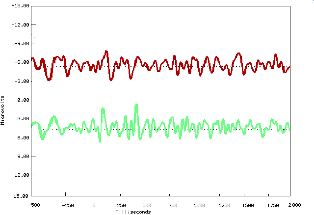
Figure 2.3a shows before rejection horizontal and vertical eye movement traces
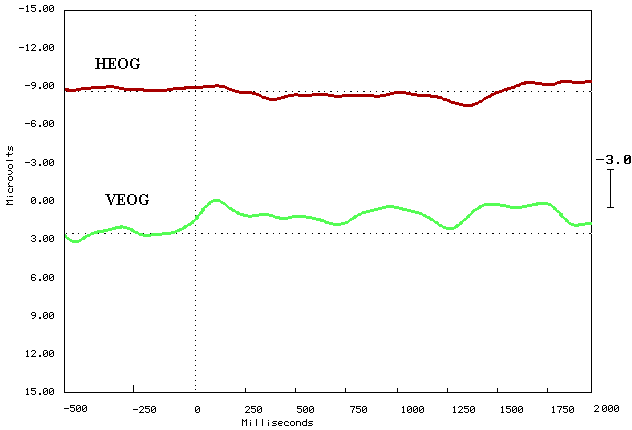
Figure 2.3b shows after rejection horizontal and vertical eye movement traces
2.10. Reference electrode
Where should the electrode be placed? We need to record the voltage difference between two electrode sites to obtain ERPs. The form in any evoked potential component is partly dependent on the choice of the reference electrode. Knowledge of the reference is of fundamental importance when interpreting waveforms, and the difficulty of finding a true reference is an important issue.
The most glaring errors in interpreting ERPs appear to originate from a misunderstanding of the reference electrode in scalp recording. Distribution or topography across the scalp recording array has always been one of the criteria for component identification. Because each 'active' scalp site is referred to a common reference, scalp distribution will depend on the location of the reference. An ideal reference site is one that is immune to brain activity (inactive).
The most common reference procedure uses a non-cephalic electrode (e.g., Erb's point) as an 'inactive' site. While the other inputs, are from electrodes over or near an 'active' area. It is important that the reference site is not influenced by the spatial field of the evoked potential or at least only minimally. So, it is clear that none of the more commonly used cephalic reference sites, such as the mastoid (bony process right behind the ear), the inion, the earlobe, the chin or the nose is completely insulated from brain activity. However, there is no electrically silent reference and no true reference electrode. It is also important to note that extra-cephalic reference can avoid brain potential contamination but it introduces heart and muscle electrical activities.
Recently much effort has done into the development of procedures for obtaining reference free estimates of the ERP and several have been created. One solution is to connect all active electrodes through resistors of equal value, to a single point, which is then used as an average reference. In this case, the reference for any given site is the average activity across all the other recorded sites. The advantage of this method is that it does not favour any particular electrode site (Bertrand et al. 1985).
There is another reference-free procedure, which provides, instead of the standard voltage measure, an estimate of the instantaneous electrical current flowing into and out of the scalp at each recording site.
Current source density (CSD) analysis is another method (Nunez, 1981, 1990). CSD is often used in combination with a spherical spline function to interpolate data recorded from irregularly spaced electrodes and to infer current sources that are not directly beneath a recording site. However CSD, like the average reference procedure, requires good spatial sampling of the scalp surface (often 64 sites or more) with precisely defined loci.
ERPs recording researches have the linked ears or linked mastoids reference as a very popular reference procedure for that it deserves a very special consideration due to this popularity. The pre-existing potentials of the two ears are not average by connecting the ears or the mastoids, but rather modifies the current flow and thus potential distribution over the whole scalp. The linked mastoid was used by most of the researchers (Coles et al. 1997). Therefore I selected the same reference electrode of linked mastoid to facilitate comparison with results in the literature.
Three experimental approaches at least were described by using the term-linked mastoids:
Fortunately digital recording allows re-calculation of signal with any choice of reference after recording.
2.11. Recording Procedure: (Figure 2.4.)
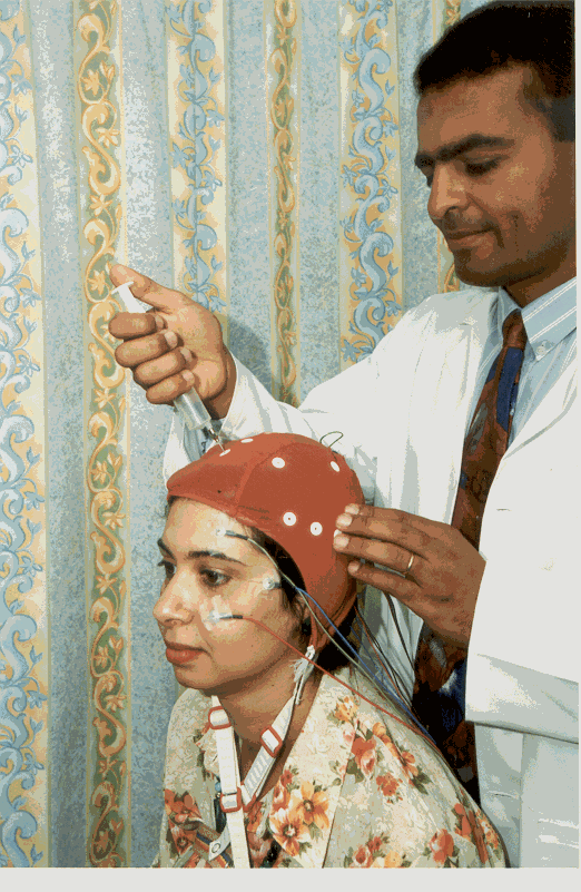
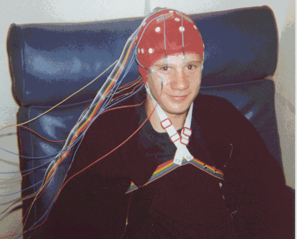
Subjects had an electrodes cap on their head hold 32 tin electrodes sites to the scalp (Figure 2.5.), Electro-cap international were designed by NASA in United States of America and made of elastic fabric which fits the geometry of the head, available in different sizes, large 58-62 cm head circumference, medium 54-58 cm head circumference, and small 46-50 cm head circumference. This cap contain 22 tin electrodes, built into small plastic buttons (0.5 cm) in an enhanced international 10/20 electrode placement system (Jasper, 1958). They did not use the more common silver electrodes, because it would be impractical for silver to be imbedded in a cap, as it needs to be regularly chlorided to prevent oxidation and polarisation. Gold, silver, and platinum can be polarised, which occurs when a current passes between a pair of electrodes and causes electrolysis and produce a standing voltage between electrodes. Variation in this voltage is a source of noise and can affect the electrode’s frequency response. A non-polarisable electrode is one whose properties do not change if a current passes through, and any ion transfer that does occur can be completely reversed. Pure tin possesses the qualities necessary in an electrode material of minimal standing potential between electrodes and is non-polarising. This ensures low and constant resistant to the flow of the current.
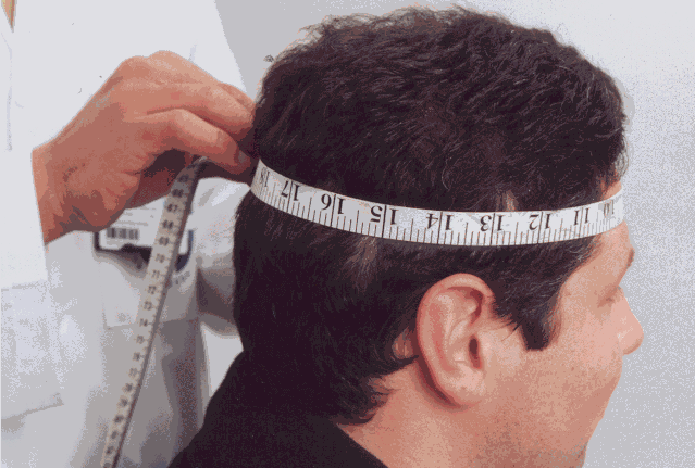
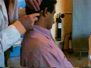
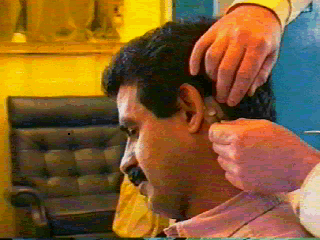
To insure the correct size of the cap, we had measured the subject’s head circumference with tape measure. Rubbing a cotton swab dipped in a suitable conductive abrasive preparation compound called SkinPure (Figure 2.6) cleaned skin electrode sites. Two tin electrodes were fixed on the subjects’ right and left mastoid, and then used as a linked reference. Electrodes were affixed with surgical adhesive tape, and Elector-gel (eci) was injected to fill the gap between the skin and the electrodes. Mastoid references are preferred for examining the distribution of cortical activity. Then the cap pulls over the head adjusted to give correct electrode placement, and fixed and secured by elastic straps from each sides of the Electro-cap to around a chest belt, to be fit secure, and avoid the discomfort feeling from fixing and securing it under the chin. The gap between the electrodes and the skin was filled and bridged with a high conductivity, non-saline electrode gel to prevent corrosion of the electrode and skin irritation, and which is formulated for use with Electro-cap system (Electro-gel. Figure 2.6.), after the skin was slightly scratched and scarified (abraded) through the hole on the top of the electrode using a blunt needle to remove the sebum or the scale and lower the impedance. Scarifying and adding the Electro-gel was continued till equal electrode impedance below 5 KW was achieved.
Electrodes are applied for long-term recording (1-1.5 hours), thus electrode gel should not contain irritants such as calcium chloride because this substance has occasionally caused skin burn and granulomatous reactions (Schoenfeld et al. 1965; and Giffin & Susskind, 1967) The locations for these electrodes include all the
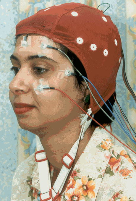
standard international 10-20 system location (Jasper, 1958) Figure 2.7. Four electrodes were affixed with surgical tape and were filled with Elector-gel for monitoring the eye movement artefact, the skin electrode site prepared by rubbing the skin with Skin Pure gel. The first couple (VEOG) above the right eye and beneath the left eye to check for eyes blinks and vertical movements. The second couple (HEOG) was placed on the outer canthus of the right and the left eye to check the lateral and horizontal movement. The impedance between each recording site and reference was reduced to below 5Kohms.
Subjects were seated in front of a computer monitor (IBM 14 inch) on a comfortable reclining chair, the chair back was high enough to allow all subjects to relax. Any tension of their head and neck muscles could interfere with our recording. The recording room was quiet, temperature controlled and dimmed (Figure 2.8.).
I asked the subject to avoid blinking except when the screen was blank. We did all our best to put the subjects at their ease.
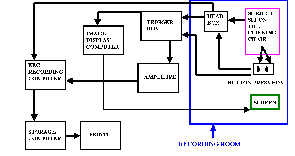
Figure (2.4.) shows the recording procedures diagram.
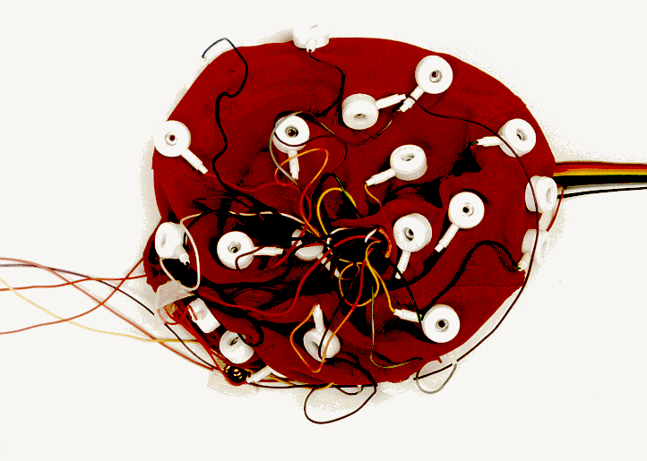
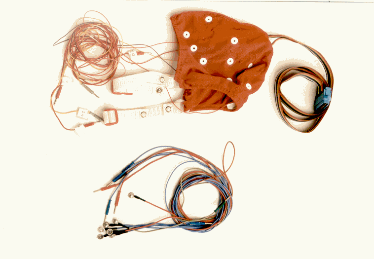
Figure (2.5.) shows my study ERPs recording cap electrode with the extra electrodes and the connecting cable to the headbox. Group of the tin electrodes
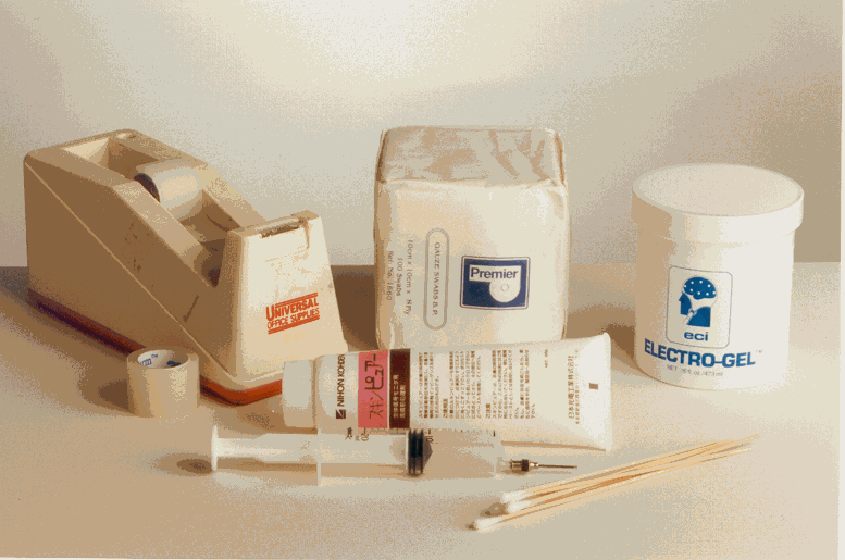
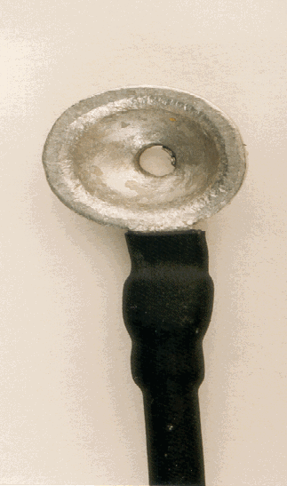
Figure (2.6.) shows my study ERPs recording materials, flexible tape measure, swabs, blunt ended needle (scarifier), syringe, electrode gel (eci), a mild skin abrasive (skin pure).
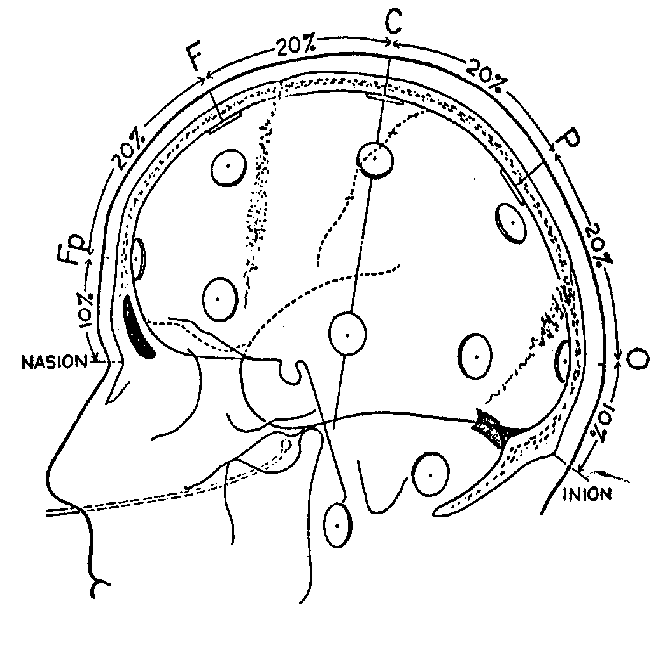
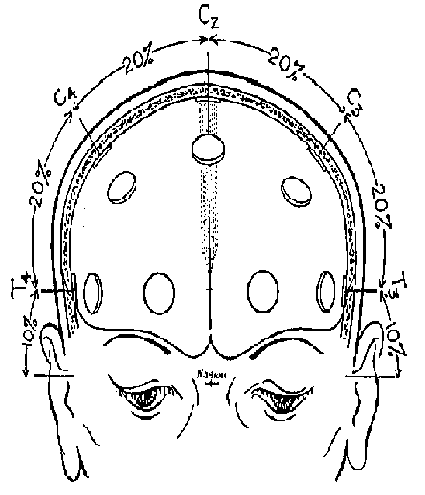
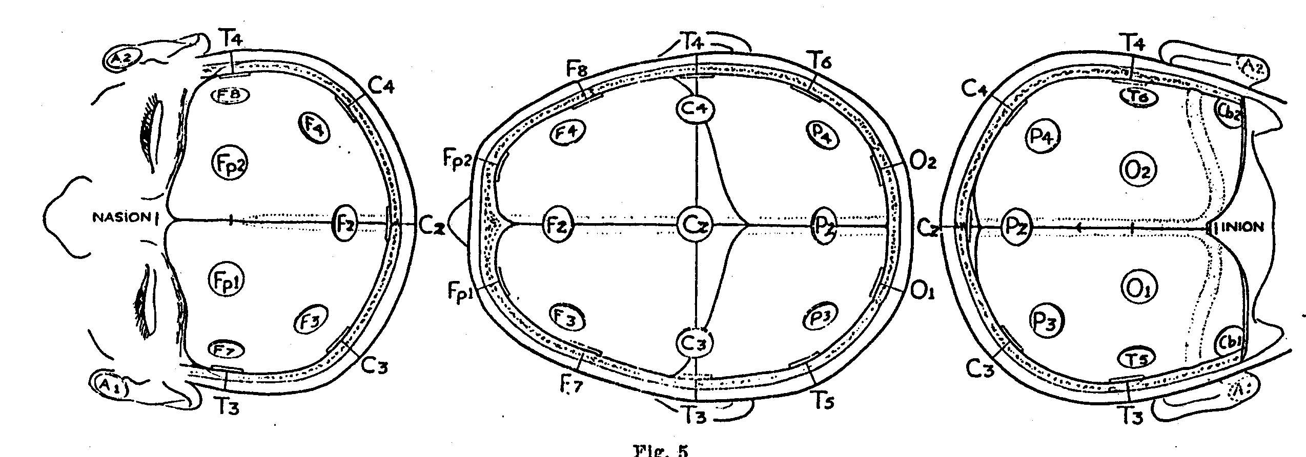
Figure (2.7.) Shows the Standard Position for placement of EEG electrodes in the 10-20 system. The abbreviation stand for A = Auricle, C = Central, F = Frontal, Fp = Frontal-pole, O = Occipital, P = Parietal, and T = Temporal. Letter Z represents the midline electrodes.
(A) (B)
(C) (D)
(E) (F)
Figure (2.8.) shows recording procedures (A) Head measurement, (B) skin preparation, (C) placement reference electrode (D) injecting the electro-gel (E) electrodes and cap electrodes placement, and (F) Subject sitting in the recording room
The electrodes and the cap could be removed without difficulty and the gel wiped off easily. We cleaned the cap thoroughly to be ready for the next recording.
All subjects completed the questionnaire after finishing the task to give us their comments about the task. (Appendix. II)
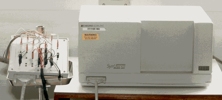
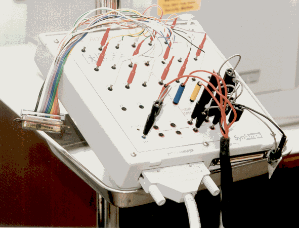
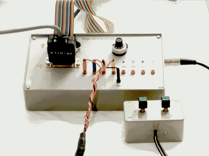
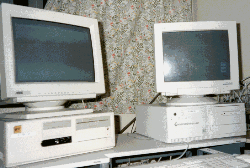
2.12. Equipment and recording systems (Figure 2.9.):
The cap electrodes discs are made of pure tin with low resistance to the current flow and good polarisation characteristics fitted to the cap by plastic rings and connected to the head box by one-meter length cable. It is a thirty-two channels head box. There are two channels for the ground, two channels for the subject response buttons and two channels for the references. It contains the first stage of amplification to reduce the effect of noise encountered during conduction into the main amplifier. The input impedance was high (15) The signals pass by shielded cable to be amplified by the SynAmps amplifiers in AC mode, containing analogue components needed to amplify the low level signals. An analogue-to-digital converter (ADC) coverted the analogue signals to digital for further processing, and was controlled by NeuroScan 3.0 (386 version 1992) software model 5083, amplifier filter bandwidth was 0.01-30.0 HZ. Further digital filtering could be applied.
Personal computer GATEWAY2000 displayed the stimuli and was linked to a specially designed box (trigger box), which was also linked to a channel of the amplifier. The trigger box required the timing, and categorisation of the stimuli and the subject responses to a second computer, which ran the NeuroScan acquisition software. This recording EEG computer was linked to extra computer used as a storage unit for the raw EEG and averaged ERPs. Coloured printer (HP Desk Jet 550) was connected to both computers to produce a hard copy of the results.
(A) (B) (C)
(D) (E)
Figure 2.9. Shows recording equipment’s (A) the head box (B) the trigger box (C) the head box connected to the amplifier, (D) zoom to one tin electrode cup, and (E) EEG and Pattern Computers
2.13. The acquisition value: (Figure 2.10.)
The EEG was digitised at 4 ms per point for 630 points and time-locked to stimulus presentation. This gave individual epoch recording from -500 msec. to 2020 msec. Thus a 2520 msec recording. With 500 msec pre-stimulus baseline.
Sweeps in which the EEG exceeded ± 70m n were manually rejected (2%); post recording baseline correction between -200 ms. and 0 ms. was applied to individual average files.
The signal filtering capabilities required depend on the frequency component of the signal. Approximate values of 1, 5, 10, 25, 100, and 300 Hz should be available as low cut-off (high pass) and 100, 250, 500, 1000, and 3000 Hz should be available as high cut-off (low pass) filters. To record the endogenous event-related potentials 0.3 to 1-Hz high pass and 30.0 to 100.0 Hz low pass filters are commonly used. We used 0.3 Hz high pass and 30.0 Hz low pass.
Another problem that can arise concerns sampling. The input waveform is sampled at constant intervals along the time scale. The number of points used for sampling or the sampling rate (points per sec) is an important parameter in digitisation. If it is incorrect aliasing can occur. This effect can be illustrated in western movies. The film camera samples the visual scene at some fixed rate, each sample occupying one frame of the film. If a wagon wheel is rotating slowly enough, the motion is reproduced faithfully, but at higher rates of motion the wheel may appear to rotate more slowly than its actual rate and may even appear to rotate backward. The false rotation speeds are generated because the movie camera's sampling rate is too low to accurately record high rate of rotation.
Similar considerations apply to the sampled EEG waveform. Errors will result unless the sampling rate is more than twice the highest frequency present in the EEG. This minimum sampling rate requirement is known as "the Nyqvist criterion". Inadequate sampling introduces an "alias' error if the frequency content of the input signal is too high in relation to the sampling rate; the Nyqvist theorem requires that the rate of sampling must be at least twice the highest frequency in the analogue signal. In practice it is better to have an even higher sampling rate than the theoretical one.
A third potential problem concerns high frequency cut-off amplifiers. Unlike the short latency responses to auditory or somatosensory stimuli, the late components themselves have comparatively low frequency (e.g. P300) or even slow potential waves lasting for second rather than milliseconds (e.g. CNV). The consequences of having a time constant that is too short are a reduction in the amplitude of the component and a shortening of its latency, thereby distorting its true value. The choice of high frequency cut-off amplifiers is also different from that for sensory evoked potentials. Many investigators record with a cut off less than 50 or 60 Hz, thus avoiding possible problems with main interference while adequately characterising the ERPs.
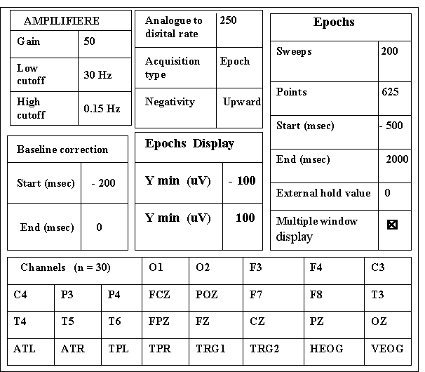
Figure 2.10. Shows the recording acquisition value.
2.14. Noise and interference
Methods of recording and measuring very small signals such as ERPs are basically procedures for eliminating noise (defined as undesired signals). Event-related recording requires separation of the nervous system's responses from accompanying noises. In ERP recording the three major sources of noises are:
1) The electrical environment (nearby AC voltage sources, such as main-powered lights and main cables), and magnetic or radiated interference.
2) Internal instrumental noise e.g. amplifier noises.
3) Biological noises: examples of such artefacts are those resulting from main pulses, eye movements, eye blinks, the activity of facial muscles, tongue movement or movement of the subject (myogenic electrical activity). These artefacts fall into two classes:
a) Those that are not time-locked to the stimulus.
h) Those that are time-locked to the stimulus.
Commercial averagers are often provided with an artefact reject mode of operation. This mode cuts out any trials with unusually large voltage. The ability of modern equipment to extract a hidden signal from noise is indeed impressive, but it is a dangerous mistake to overestimate the equipment's ability to reject non-signals.
Prevention is by far the best approach when dealing with noise and artefacts: clean inputs are preferable to noisy inputs. Rather than relying entirely on the computer, it can be enormously to one's advantage to decrease both the number of artefact-contaminated trials and the degree of contamination by carefully instructing the subject to relax and to blink as little as possible during the recording, and ensuring that the subject is truly comfortable. For example, if a chair is used, the correct height is crucial.
2.15. Average
The electrical response of the brain to the stimulus always occurs at the same interval after the stimulus, whereas the background electrical activity is not coupled to the stimulus. Averages will extract the desired ERP waveform from the random background noise (Chiappa, 1982). This technique makes a significant improvement of the signal-to-noise ratio and permits the recording of very small ERPs.
The principal of averaging method is similar to the superimposition technique, which was used more than a century ago by Galton. One of his aims was to identify common features in the faces of murderers and violent criminals.
It was the practical problem of recording reliable somatosensory ERPs in myoclonic epilepsy that led Dawson to use the superimposition technique of signal-to noise enhancement in ERP recording. Using the statistical theory of averaging he created a powerful practical tool, known as an automatic signal averager, which he demonstrated to the Physiological Society in May 1951 (Dawson, 1951). Dawson's automatic signal averager can be seen in the Science Museum in London.
With the advent of computer averaging, it became possible to obtain an estimate of activity, which is time-locked to an arbitrary point, such as the onset of a stimulus. At the scalp an event related potentials (1-20 microvolts) is substantially smaller in amplitude than the background EEG (50-100 microvolts) and must, therefore, be extracted by an averaging procedure using software such as NeuroScan. This involves recording ERPs for repeated presentation of 'similar' stimuli. Each stimulus is recorded as a discrete 'sweep' lasting a few seconds each. Once enough of the same type has been recorded they can be averaged together. To record late event-related potentials, fewer than 25-30 trials on average do not usually provide a good signal-to-noise ratio (Kutas & Van Petten, 1990). However, as the number of sweeps is increased the ERP waveform becomes easier to distinguish from the background activity. Fifty or more sweeps have been averaged usually in my work.
The mainstay-evoked potential signal processing is averaging. The stimulus is presented many times and the EEG signals for the duration of interest immediately following are summed and then divided by the number of presentations to obtain the average evoked potentials as shown here and in the equation, the ‘n’ is the number of sweeps.
S/N
µ Ö nThis technique makes a significant improvement of the signal-to-noise ratio and perm to the recording of very small-evoked potentials.
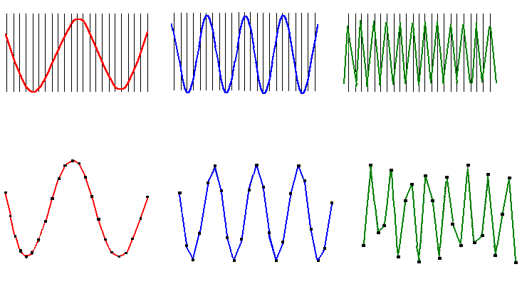
Figure 2.11. Shows the relation between the sampling rate and the signal frequency. The sampling rate must be at least double the fastest signal of interest frequency.
2.16. BRAIN MAPPING
The goal of the brain mapping is to isolate local neural activity associated with sensory, motor, and cognitive functions. The current flow either into or out of a cell through charged neuronal membranes generate the ongoing EEG. The EEG recorded at the scalp is largely attributable to graded postsynaptic potentials (PSPs) of the cell body and large dendrites of vertically oriented pyramidal cells in cortical layers three to five (Lopes da Silva, 1991). These synaptic potentials are of much lower voltage than action potentials, but they also last much longer and involve a larger amount of surface area on cellular membranes and, as a result, the extracellular current flow produced by their generation has a relatively wide distribution. Several factors determine the degree to which a cortical potential will be recordable at the scalp, including the amplitude of the signal at the cortex, the size of a region over which PSPs are occurring in a synchronous fashion, the proportion of cells in that region which are in synchrony, the location and orientation of the cells in relation to the scalp surface, and the amount of signal attenuation and spatial smearing produced by conduction through the intervening tissue layers of the dura, skull, scalp. PSPs are thought to be synchronised by rhythmic discharge from thalamic nuclei (Lopes Da Silva, 1991), with the degree of synchronisation of the underlying cortical activity reflected in the amplitude of the EEG recorded at the scalp.
2.16. NeuroScan
NeuroScan software (version 386 and version 4.0.30) was used to record and display of the data. This program is divided into six sub-modules as shown in (Figure 2.12. & 2.13.). Each module performs a different function on the data: Acquisition and on-line processing is performed by Acquire program; Topographic mapping by Window program; Statistical analysis by Stats program; map template construction by Mapgen program, retrieve raw data, viewing and edit by Edit program and image editing by Draw program.
The NeuroScan Acquire program records averaged, epoch, and continuous EEG data from up to 64 channels with the scan system. The collection of data mainly done by the general steps, first step is to select a set-up file to configure the system (set individual parameters related to data acquisition), then number two enter subject information and finally acquire (and save) the data.
The NeuroScan Edit program performs a variety of off-line modifications to EEG data attained by the acquire program. Mainly used for averaging after observing all the sweeps one by one by eye, then rejection done for contaminated trials by eye-movement, muscle, or amplifier saturation artefacts. Baseline correction was set for -200 msec to 0 msec.

Figure 2.12
. Shows Neuroscan version 3.0

Figure 2.13. Shows NeuroScan version 4.0
The ERPs were averaged for each subject in each needed condition (all the trials, First and last fifty trials, Correct and incorrect trials, and for the pattern A & B trials). Over an epoch beginning 500 msec before stimulus onset and extending 2000 msec post-onset. The stimuli were exposed for 2000 msec on a computer monitor, and the interval time between them was 2000 msec and saved.
The NeuroScan WINDOW program topographic mapping package in colour or black and white, can map the averaged sweeps or single sweep of the recording data. This technique of the topographic mapping for displaying the waveform data from large multi-electrode arrays. The results are a multicolour surface that represents the scalp distribution of voltage. The general idea is to take an array of electrodes, e.g., the 10-20 system, and place this array on a computer-generated surface. The WINDOW program (part of Neuro-scan) applies a colour gradient to a range of voltage (or other computed statistic) amplitudes represented at all electrodes. With mapping, the voltage values are displayed on a surface in the form of colour intensity gradients. Since there are typically fewer electrodes than points on the surface, missing values between the individual electrodes are ‘filled in’ with an interpolation algorithm. Then, the greater the number of electrodes used to cover the scalp, the smaller the inter-electrode spacing, and the greater the spatial resolution. The result is a multi-coloured surface that represents the scalp distribution of voltage. Basically there are four methods can be displayed by which the map in NeuroScan. Animated maps can be made into movies, which are played back on the computer screen. Cartoon maps of each msec. for a given time window can sequentially be displayed and run in several pages and can also be scrolled through, the cartoon series of small maps each corresponding to a short segment of large time window from the averaged waveform and show evolution of potentials. A large map can also be made for specific time range. These maps can be shown with or without the electrodes superimposed, by placing the cursor anywhere we can map at any latency. To study the potentials we were using the top view, right view, and left view. The scale is always shown to the right-hand side of the cartoons or large map figures, in the form of colour intensity gradient. Brain activities can be highlighted in different scale because these maps depend on the potentials scale factor. Maps show spatial and temporal changes, but the comparison is qualitative rather than quantitative, and it is useful method for combining the information from multi-channel recording.
Large maps and cartoon maps were used (Figures 2.14a and 2.14b). A large map is a full-sized map of a waveform over an interval of time. The cartoon is a series of small maps, each corresponding to a short segment of a larger time interval for a waveform average file and shows the evolution of potentials. The colour scale represents the maximum and minimum amplitudes and all other intervening amplitudes.
The rationale for topographic mapping is that the traditional EEG or ERP tracings contain information, which under normal circumstances is not observable by the naked eye. This is because there is simply too much data in a form unsuited for visual analysis. In this instance, the solution is to apply mathematical processing for interpolation of data to derive spatial bitmaps. To discern the interrelationships between different scalp locations, one can merely arrange such a plot in a manner so as to mimic a head diagram. This results in a two-dimensional spatial bitmap. In the MAPGEN program, the window can display data on mapping templates created by the user.
The NeuroScan MAPGEN program general purposes map template generation and editing. The program uses a shape created with the draw screen editor as a surface for mapping template, this mapping template contains information about the location of the electrodes in addition to the surface, and it is used by window program to construct topographic maps of waveforms and spectral data. I draw my own electrodes configurations for the top, right hand side electrodes, left hand side view to give me the opportunity to use WINDOW program to process my volunteers brainmaps.
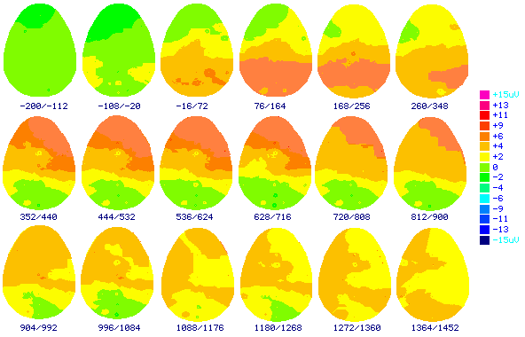
Figure 2.14a. Shows right-hand side view large brainmap. The maximum and minimum amplitudes and all other intervening amplitudes represented by the colour scale.
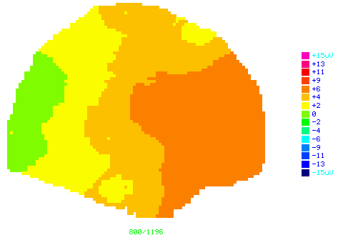
Figure 2.14b. Shows top view cartoon brainmaps. The maximum and minimum amplitudes and all other intervening amplitudes represented by the colour scale.
The NeuroScan STAT program is designed as an exploratory data analysis tool for first look at statistical comparison creating group average waveforms. Comparing two group-averaged waveforms, comparing individual average waveforms with group averaged waveform, comparing two individual average waveforms. Import of ASCII data files obtained from another acquisition system for further analysis. Export scans averaged files to ASCII files format. Subtraction of two groups averaged waveforms and left hand side and right hand side averaged waveforms.
2.18. Statistical Analysis:
There were many quantitative measures and statistical procedures available. The files can be exported to other programs for required analysis. Before embarking on analysis I had to access the subjects’ performance.
2.18.1 The subjects’ performance learning was accessed by CUSUM statistical method:
Industrial processes were monitored by the developed control chart during the 1930’s, the important processes control parameters (mean or standard deviation) of sequences of random variables were plotted in simple graphs versus time, or the number of items produced (De Bruyn, 1968; Royston, 1992).
The CUSUM (Cumulative Sum) technique is among simplest statistical manoeuvre available that makes possible rapid analysis, identification, and powerful assessment of trends in a series of data (De Saintaoge et al, 1974; Kinsey et al, 1989). The cusum assessment is retrospective, not prospective (Robinson et al 1974).
More recently, CUSUM was used by several researchers to do rapid, and accurate evaluation for variables such as, surgical trainee performances (Van Rij et al, 1995), sigmoidoscopy results of novices performances in comparison with experienced personnel (Williams et al, 1992). There is no universally accepted method of quantifying circadian blood pressure patterns, but the cusum is a valuable methods for circadian blood pressure assessment (Staton et al, 1992), also measuring the competence of anaesthetic trainees at practical procedures (Kestin, 1995). Retrospective analysis by cusum plots conventional temperature charts of neutropenic patients (Kinsey et al 1989), pregnancy, death, recurrence of diseases, and so on, occur commonly in medicine.
The CUSUM starts at zero, increasing in the cusum trend indicate success (figure 2.15), and a declining in the cusum trend indicate failure (Figure 2.16). We have derived learning curves from the results of the random visual stimulus experiment, by assigning the value 1.0 to each success, and the value 0.0 to each failure. As the performance of the subject is seldom perfect, it is usual to allow a certain tolerance e.g. a 10% (0.1) failure rate. A subject performance with 90% success will generate an upward line and the line will move downward for a worse performance. Individual increments for the cusum would then be 1.0 - 0.1 = 0.9 for each success, and 0 - 0.1 = -0.1 for each failure.
This may be express mathematically as: - CUSUM (i) =
å (Result (i) - Tolerance)The results were analysed, and curves plotted, using the MathCad computer aided design software package (MathSoft).
We set our tolerance at 30%. Subjects learning within this tolerance produce ascending line, subjects not learning produce a descending line (Figures 2.15 & 2.16.)
Connectionally, at the beginning of measurement, the CUSUM start at zero. With a successful process the CUSUM increases to positive value, with failure it declines to more negative value.
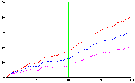
Figure 2.15. Shows learner’s performance. Tolerance 10% (0.1) failure rate in red line, tolerance 20 % blue line, and tolerance 30% pink line. Y-axis: represents the performance. X-axis: represents the 200 trials.
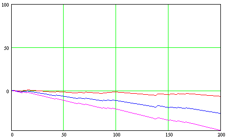
Figure 2.16. Shows non-learner's performance. Tolerance 10% (0.1) failure rate in red line, tolerance 20 % blue line, and tolerance 30% pink line. Y-axis: represents the performance. X-axis: represents the 200 trials.
2.18.2. Decision time statistical analysis:
Each subjects decision time and performance for each experimental condition in both groups (learners group and non-learners group), logging (text) files were transferred to the Statistical Package for the Social Sciences (SPSS). Then Mean maximum value, minimum value, and standard deviation (SD), have been quantified and compared for each one of these conditions all the task subjects decision time. Beginning of the task (first fifty), end of the task (last 50). Correct, incorrect trials subject’s decision times and patterns A, and pattern B as well
2.18.3. Event related potentials statistical analysis:
I have grand averaged for learners group and non-learners group, the correct & incorrect answer trials sweeps, and first fifty & last fifty sweeps; the ERPs were measured, quantified & compared. There are some common methods to measure the amplitude and the most commonly used are these two which called "absolute amplitude". First is "baseline to Peak" but sometimes it is difficult to define the base line, which make this more subjective method than the second one. Second one is "Peak to peak" by measuring the peak of one polarity to the immediately following peak of the opposite polarity. Because of the activity producing the first polarity may have nothing to do with the immediately following peak of the opposite polarity so it looks like mixing apple with orange. Area measurement is another method, which is theoretically the most sensible technique and effectively can be done by using the computers. To be more accurate I chose the most commonly used method in this same research area. The mean amplitudes were calculated, by using the mean value of many points within a time window. The windows which extend from the beginning to the end of the target or desired component. The first time window was (250 msec to 500 msec) after the stimulus and the second time window was (500 msec to 800 msec) after the stimulus and both of them is 75 sampled points.
Table (2.2a & 2.2b) shows an example of the results of repeated measures, the mean square (MS) shown in the fourth column which is obtained by dividing each of sum of squares (SS) by the degree of freedom. Hypothesis tests are based on the ratios of each source of variation mean squares to the residual mean square. The larger the F value, the smaller the observed significant level (£ 0.05) and indicate that the hypothesis that the constant is zero is rejected.
|
Source of Variation |
SS |
DF |
MS |
F |
Significance of F |
|
Location |
264.185 |
(8,112) |
33.023 |
2.18 |
0.034 |
|
(greenhouse-Geisser) |
264.185 |
1.896 |
139.354 |
2.18 |
0.01 |
Table (2.2.2.) shows the significance of F value before and after using the greenhouse-Geisser for location within subjects effect. p *
£ 0.05, ** £ 0.01, *** £ 0.001.The following table (2.2.3.) are an example of testing interaction. The F value associated with the group and electrodes locations is 20.60 and the significant level by considering Greenhouse-Giesser correction is 0.135, therefore, it appears that there is not an interaction between group and locations.
|
Source of Variation |
SS |
DF |
MS |
F |
Sig. Of f |
|
Group X Locations |
489.560 |
24 |
20.398 |
20.60 |
0.324 |
|
(greenhouse-Geisser) |
489.560 |
2.412 |
202.943 |
2.060 |
0.135 |
Table (2.2.3.) shows the significance of F value before and after using the greenhouse-Geisser by using two ways ANOVAS (group X location within subjects). p *
£ 0.05, ** £ 0.01, *** £ 0.001.Latency and amplitude increase and decrease were studied and assessed by inspection through the event related potentials waves morphology (positive and negative deflections), comparison was made between the averaged all sweeps, correct & incorrect responses sweeps, first & last 50 sweeps, and right and left side sweeps too.
Most of the statistical results obtained from my experiments are presented as tables and Error Bar charts that plot the mean value of data, the confidence intervals, standard error, or standard deviations of individual variables. I have chosen Error Bar charts for many reasons. Firstly, they can show summaries for groups of cases or summaries of separate variables and can be simple or clustered. Secondly, they can present three different types of statistics: confidence intervals, standard errors, or standard deviations. 1 have chose the 95% confidence interval, which reaches approximately two standard deviations on either side of the mean.
2.19. Experiments:
2.19.1. Experiments 1: with feedback and without rule (Fr)
2.19.1.1. Subjects:
The subjects were 34 young adult volunteers (15 females & 19 males) participate in the same task, aged 21:34 years.
2.19.1.2. Task:
Subjects were asked to make a single response as promptly and accurately as possible to each image within the image display time (2-sec.). As soon they pressed one of two buttons A or B according to his/her decision and we gave them screen message feedback ‘Right’ (Figure 2.17a) or ‘Wrong’ (Figure 2.17b) directly
without delay. Feedback may be defined as any signal to a learner, which indicates the correctness or incorrectness of his previous response (Bourne, et al. 1971).

Figure 2.17a. Shows image type A when displayed and feedback is correct as shown according to the subject response.

Figure 2.17b. Shows image type B when displayed and feedback is incorrect shown according to the subject response.
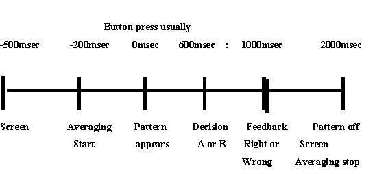
2.19.1.3. TRIAL
2.19.2. Experiment 2: with feedback and with rule (FR)
2.19.2.1. Subjects:
The subjects were 15 young adult volunteers (7 females & 8 males), participated, aged 18: 24 years (mean 21.13 ± 2.23).
2.19.2.2. Task:
All information’s (explicit information) were given for these subjects about all the details of the pattern contents, and the differences between both patterns, simply telling them what is going on. 200 images of pattern A & B were displayed randomly for these subjects. Subjects were asked to watch the screen and find out the differences between the both patterns and making decision by pressing one of two buttons. We gave them feedback (right) or (wrong) according to them decision.
2.19.3. EXPERIMENT 3: without feedback and without rule (fr)
2.19.3.1. Subjects:
The subjects were 24 young adult volunteers (10 females & 14 males) participate in the same task, aged 19: 28 years.
2.19.3.2. Task:
Subject made a single response to each image as soon as possible within the image display time (2 sec.) by pressing the mouse button A or B according to his/her decision and we did not give them screen message feedback (guessing group).
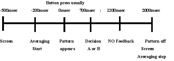
2.19.3.3. TRIAL
2.19.4. Experiment 4: without feedback and with rule (fR)
2.19.4.1. Subjects:
The subjects were 15 young adult volunteers (7 females & 8 males), participated, aged 18: 24 years.
2.19.4.2. Task
All information’s (explicit information) given for these subjects about all the details of the images contents, and the differences between both patterns. 200 images of pattern A & B were displayed randomly for these subjects. Subjects were asked to watch the screen and find out the differences between the both patterns and making decision by pressing one of two buttons, but feedback was not given to them.
2.19.5. Experiment 5: Observers
2.19.5.1. Subjects
The subjects were 11 young adult volunteers (5 females & 6 males) participate in the same task, aged 18: 30 years.
2.19.5.2. Task
The same patterns (A & B), and all the same image numbers (200) were displayed for these subjects. Subjects were just asked to watch the screen without either decision making or pressing buttons (Passive Group).
2.19.5.3. TRIAL: