Stray field calculation through analytical techniques

Alternatively, we can interpret the discrete magnetisation vector $\ensuremath{\mathbf{M}}(\ensuremath{\mathbf{r}})$ at the surface of the sample as a layer of dipoles and compute the stray field at the MFM tip and consequently the second derivative analytically.

This approach is more accurate in determining the second derivative because $h$ in equation 6.6 cannot be made arbitrarily small. Additionally, an analytical approach is more flexible with respect to the fly height of the MFM tip.

It should be noted that this approach ignores the higher order magnetic moments associated with each simulation cell in OOMMF by replacing them with the leading dipole term. This is justified if the height of the MFM tip above the sample surface is much greater than the OOMMF cell spacing.

Figure 6.8: Microscopic images of an antidot array. The tunnelling image on the left shows the location of the antidots; the magnetic force microscopy image on the right highlights the demagnetisation field

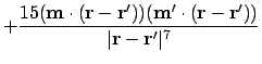
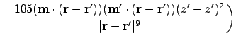
The second derivative of the demagnetising energy should be proportional to the signal at the tip of a magnetic force microscope and can be shown (see appendix A) to be:

$${\partial^2E_d \over \partial z'^2} = {\mu_0} \left ( {-3\cdot \ensuremath{\mathbf{m}}\cdot \ensuremath... ...}}' \over \vert\ensuremath{\mathbf{r}}-\ensuremath{\mathbf{r}}'\vert^5} \right.$$

$$+ {15 \cdot \ensuremath{\mathbf{m}}\cdot \ensuremath{\mathbf{m}}' (z-z')^2 \over \vert\ensuremath{\mathbf{r}}-\ensuremath{\mathbf{r}}'\vert^7}$$

$$- {6 \cdot m'_zm_z \over \vert\ensuremath{\mathbf{r}}-\ensuremath{\mathbf{r}}'\vert^7}$$

$$+ {30 (\ensuremath{\mathbf{m}}\cdot(\ensuremath{\mathbf{r}}-\ensu... ...)m'_z(z-z') \over \vert\ensuremath{\mathbf{r}}-\ensuremath{\mathbf{r}}'\vert^7}$$

$$+ {30 (\ensuremath{\mathbf{m}}'\cdot(\ensuremath{\mathbf{r}}-\ens... ...))m_z(z-z') \over \vert\ensuremath{\mathbf{r}}-\ensuremath{\mathbf{r}}'\vert^7}$$

$$+ {15 (\ensuremath{\mathbf{m}}\cdot(\ensuremath{\mathbf{r}}-\ensu... ...thbf{r}}')) \over \vert\ensuremath{\mathbf{r}}-\ensuremath{\mathbf{r}}'\vert^7}$$

$$\left. - {105 (\ensuremath{\mathbf{m}}\cdot(\ensuremath{\mathbf{r... ...^2 \over \vert\ensuremath{\mathbf{r}}-\ensuremath{\mathbf{r}}'\vert^9} \right )$$ (6.7)

This assumes that the tip of the MFM is a dipole:

$$\ensuremath{\mathbf{m}}' = \left( \begin{array}{c} 0\\ 0\\ C \end{array} \right )$$ (6.8)

The full derivation of this can be found in appendix A.

Figure 6.9: Demagnetising field of an antidot sample in zero applied field as measured by the tip of the magnetic force microscope (left) and the second derivative as computed through the analytical techniques from equation 6.7 (right)

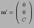
Figure 6.9 shows the comparison between the experimental data measured with a magnetic force microscope in zero applied field and the second derivative of the demagnetising field as calculated by the above equation. There is a significant similarity between the images; both show a characteristic periodic parallelogram pattern. The tip distance, both experimental and computed, was half of the distance between the antidot centres.

Figure 6.10: Measured MFM signal of a three-dimensional antidot sample in a small ($\approx$10mT) applied field (left) and simulated MFM signal of a simulated two-dimensional layer using equation 6.7 (right)

Figure 6.10 shows a clear agreement between the measurements from the MFM in a small applied field (approximately 10mT) and the computed stray field from the simulation results.

Figures 6.9 and 6.10 suggest that the simulation of a two-dimensional layer with cylindrical holes produces a magnetisation which is at least qualitatively in agreement with the measured magnetisation in the top layer of a three-dimensional sample with spherical holes.