How many cases are there in each neighpol1 category?
Before beginning any form of statistical analyses on any variables, it’s important to run frequency checks on the data contained in those variables. This is important irrespective of what type of variable you are interested in - categorical or continuous. These frequency reviews are quick and easy to do and they are enormously helpful in making sure that the variable’s data make sense and are without errors.
Frequency tabulations allow you to see how many individuals (or cases) fall into each category of the variables you are interested in. In addition, they also let you check for inconsistencies in the information entered into your variables. After you calculate frequencies, you could find that you have a lot of missing data or that missing data has been entered into the variable with numeric codes like “8” or “9,” which serve as place holders in variables when information doesn’t exist for certain individuals. This missing data could create problems in your analyses, so it’s best to search it out before you begin running tests.
To check the frequencies of the data in neighpol1, simply click on Analyze, Descriptive Statistics, and Frequencies. Find neighpol1 in the variable list on the left side of the Frequencies dialogue box and move it to the Variable(s) text box on the right. You can easily search for variable names in dialogue boxes by right-clicking on the list of variables and selecting Display Variable Names and Sort Alphabetically. (This is a trick you can use in SPSS all the time – it makes finding variables in large datasets much easier.)
When neighpol1 is in the Variable(s) text box, click OK.
Your Output table should look like the table on the right.
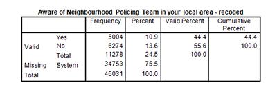
Notice that there are a total of 11,278 responses to neighpol1, and that 34,753 cases are listed as “System Missing.” Remember that in this section, we are using the Crime Survey for England and Wales (CSEW), which is a large-scale survey conducted each year in an effort to better understand public experiences with crime and the police. In the CSEW, all respondents are asked to complete a general questionnaire, and then each respondent is assigned to one of four follow-up modules, so that only about 25% of the total survey sample participates in each follow-up module. Our variable neighpol1 is a variable exclusive to Module A - only respondents in that module were asked about their awareness of neighbourhood policing. When we use this variable as our dependent variable in SPSS, we need to be careful to use explanatory (or independent) variables that have been asked either only of Module A respondents or of the entire survey sample. This same logic applies to all datasets you might analyse – always be sure that the independent variables you select contain information from the same respondents as the dependent variable you are analysing.
So, those “System Missing” cases simply represent the 75% of respondents who were not included in Module A and therefore did not provide an answer to neighpol1. These missing cases won’t create a problem, as SPSS knows to not to include them in further analysis. We also are still left with over 11,000 respondents, which is plenty to conduct good in depth analyses.
From the frequency table above, we can conclude that the data in neighpol1 is ready for use, and now we can feel comfortable using this variable in bivariate and multivariate statistical analysis.
Frequencies
Now, we’ll explore what we do if we run a frequency check and find errors.
One of the variables we might want to see is related to the awareness of neighbourhood policing is age – we may think that certain age groups are more likely to be aware than others. So, in a similar way to checking the neighbourhood policing awareness variable, we should also check age.
We can easily do this again using the Frequencies function. Select Analyze, Descriptive Statistics, and then Frequencies.
Find the variable age, and move to the Variable(s) box in the Frequencies dialogue box.
The Output window should provide you with a large output box detailing the number of cases in each age, 16 through 105, just like the one on the right. At the very bottom of this output box, however, you’ll find “998” and “999” entered as age categories.
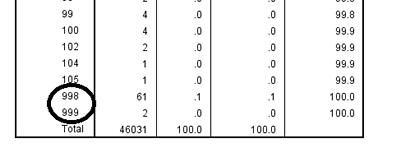
This is obviously an error, as it isn’t possible that any of the human respondents to the CSEW were nearly 1,000 years old. Why has this happened? Sometimes, all missing values in a dataset, regardless of variable type, are given numeric codes such as “998” or “999.” We are going to have to tell SPSS to remove these missing values from future analysis, because this enormous age maximum could really alter the outcome of our analyses, as it spreads the range of our age data out over nearly nine hundred more years than it should.
However, before we remove the missing values, let’s run some descriptive statistics on the variable age. We can repeat these steps again when we have finished “cleaning” age to see the difference made by the removal of the missing values.
Select Analyze, Descriptive Statistics, and then Descriptives.
Find the variable age, and move it over to the Variable(s) box. Click OK.
Your output should look like the one on the left.
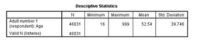
This output box lists the number of respondents (N), the minimum and maximum values of responses, the mean value, and the standard deviation, which is a statistic that tells us how much the data varies around the mean. Note that for age we have over 46,000 respondents – everybody in the dataset was asked this question – not just a quarter like before.
And you can see that the maximum age included above is 999, which is totally nonsensical and influences the value for the mean and the standard deviation.
So, now let’s focus on removing those missing values from the data.
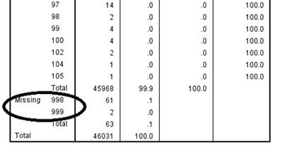
You can see in the age frequency table above that there are only sixty-three missing “998” and “999” values here (out of our total sample size of 46,031). Because the number of missing values is relatively low in relation to the total number of cases, it is alright for us to remove them from the analysis of our variable (if there was a larger percentage we may be worried about doing this). It is quite easy to remove them. Find the variable age in the Variable View window. Notice that at the far right of the window, there is a column called Missing. This column codes variable values as “missing values,” therefore preventing them from being included in analyses performed on the variable. All we need to do now is enter in “998” and “999” into the Missing cell in the variable age row, and these numeric values will not be included in further analyses of age.
To add “998” and “999” as missing values for the variable age, just double click on None in the Missing cell on in the age row. Click on the ellipses that pop up next to the word None.
Select Discrete missing values and enter in “998” and “999,”as these are the numeric codes for missing values that we want SPSS to recognize as not part of the sample data.
Click OK. You should now see “998” and “999” in the Missing cell of the age row.
Now we can check the frequencies of age to see if we have successfully coded “998” and “999” as missing values. Select Analyze, Descriptive Statistics, and then Frequencies. Move age to the Variable(s) text box and click OK. Now, you should see that the age range ends at 105, and that 998 and 999 are coded as missing values. Check the output table on the right to be sure.
Let’s check to see if this recoding of “998” and “999” had any effect on the descriptive statistics for the variable age.
Now we can select Analyze, Descriptive Statistics, and Descriptives once more. Our variable age should still be selected in the dialogue box, but if it is not, find it and move it over to the right side of the box. Click OK.
The maximum respondent age in this new round of descriptive statistics is 105, just what we would expect. In addition, both the mean and the standard deviation have changed with the removal of the “998” and “999” values. Before we filtered out the missing values, our age mean was 52.54 and our standard deviation was 39.746. How our age mean is 51.24 and our standard deviation is 18.84 - quite a large difference. Therefore, by filtering out the missing values, we have prevented our data from being unnecessarily compromised.
Summary
In this section you have studied the variable related to your research question – awareness of neighbourhood policing – and investigated if there was missing data. You have also checked the frequencies of the data in the variable age and successfully recoded the missing data in the age variable so that it can no longer skew later analyses.
Note: as we are making changes to a dataset we’ll continue using for the rest of this section, please make sure to save your changes before you close down SPSS. This will save you having to repeat sections you’ve already completed.