We’ve seen in the previous section that employment status has a significant influence on the odds of neighbourhood policing awareness. We might also be interested in the relationship between educational attainment and awareness. However, because respondent employment status may be informed by respondent educational qualification, it is best if we fit another logistic regression model, using
neighpol1
as the dependent variable and entering both
remploy
and
educat3
, a second categorical independent variable measuring respondent education level, as the independent variables at the same time.
Select
Analyze
,
Regression
, and then
Binary Logistic
.
Make sure that
neighpol1
is in the
Dependent
box and
remploy(Cat)
is in the
Covariates
box. Find
educat3
in the variable list on the left and add it to the
Covariates
box.
Because
educat3
is another categorical variable, we need to have SPSS create dummy variables. Click on
Categorical
in the upper right corner of the
Logistic Regression
dialogue box.
Move
educat3
to the
Categorical Covariates
box on the right.
Click
Continue
.
You should now see both
remploy(Cat)
and
educat3(Cat)
in the
Logistic Regression
dialogue box. Click
OK
.
Now we can look over the output of our new logistic regression model.
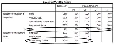
In the
Categorical Variables Codings
table, you can see that our two categorical variables,
remploy
and
educat3
, have been recoded into dummy variables. In
educat3
, the baseline variable is
Other
. You can tell this because
Other
has not been coded as “1” in any of the
Parameter Code
columns. In
remploy
,
Economically Inactive
is again the baseline variable. We will need this information when we want to analyse the odds ratios.
Again, just as we did in the previous logistic regression, we’ve left out the output tables for
Block 0
. We won’t need them in our analysis. (If you would like to work through the information in these tables, please go to the
Simple Logistic Regression - One Continuous Variable: Age
page in this section.)
Now we can look at our Block 1: Method = Enter output tables, which will display the results of our multiple logistic regression.
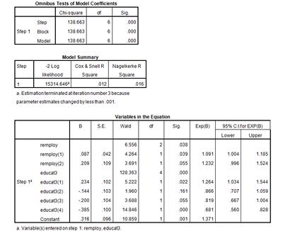
Does this final model have a better fit than the previous two logistic regression models we created? Looking at the output in the Model Summary table, we can see that the Cox & Snell r 2 has risen from 0.001, its value in both of our previous logistic regressions, to 0.012 in this multiple logistic regression (meaning that 1.2% of the variation in neighbourhood policing awareness can be explained by this model). Therefore, this model has a better fit than our previous two simple logistic regression models.
Examining the
Block 1
output, we can see what (if anything) has changed in the predicted odds of being employed and unaware of neighbourhood policing, now that the model controls for education level. Remember that in this model, “Economically Inactive” was selected as our baseline comparison dummy variable and is called
remploy
in our model outputs. Because
remploy(1)
(with a p-value of .039) is a significant predictor of the odds of neighbourhood policing awareness, we can use the odds ratio information provided for us in the
Exp(B)
column to say that a respondent who is employed has odds of being unaware of neighbourhood policing that are 1.091 of the odds of someone who is economically inactive. We can compare that result to 0.917, the odds ratio for an employed respondent being unaware of neighbourhood policing we found in our previous logistic regression. Because the odds ratio for employed respondents is now greater than 1, this model predicts that the employed are now
less
likely than the economically inactive to know about neighbourhood policing. An odds ratio less than 1 means that the odds of an event occurring are lower in that category than the odds of the event occurring in the baseline comparison variable. An odds ratio more than 1 means that the odds of an event occurring are higher in that category than the odds of the event occurring in the baseline comparison variable.
This change in neighbourhood policing awareness in people who are employed is reflected in the
B
(or log-odds) column of the
Variables in the Equation
table. In our previous simple logistic regression of
neighpol1
and
remploy
, the
B
coefficient for
remploy(1)
(or employed respondents) was -0.086, meaning that the odds of an employed person being unaware of neighbourhood policing were lower than those of an economically inactive person. Now, however, the
B
coefficient for
remploy(1)
is 0.087, meaning that in this multiple logistic regression that controls for education level, the odds of an employed person being unaware of neighbourhood policing are now higher than those of an economically inactive person.
It can be quite confusing that the relationship between variables changes from a positive one (i.e. employed people are more likely to be aware) to a negative one (i.e. employed people are less likely to be aware) when we run a model twice with different variables. However, this just means that when we take out the effect of education, the relationship between neighbourhood policing and employment is the other way around. We are now calculating the relationship between employment and awareness of community policing while controlling for the effect of education.
Summary
Here, you’ve run a multiple logistic regression using neighpol1 as a binary categorical dependent variable and both educat3 and remploy as categorical independent variables. Using the output of this multiple logistic regression, you predicted the odds of a survey respondent being employed and unaware of neighbourhood policing, much like you did in the previous logistic regression including only neighpol1 and remploy. You were able determine how these predicted odds changed after you added educat3 to the model and controlled for the influence of respondent education.