What are the odds that a young person will not be enrolled in full time education after secondary school, taking Year 11 placement satisfaction and total GCSE score into consideration?
We’ve seen in our two previous logistic regression models that total GCSE score in Year 11 and satisfaction with work, education, or training placement in Sweep 1 each have statistically significant relationships with full time education enrolment after secondary school. However, our previous logistic regression models explored the influence of each of our independent variables individually. Because respondent placement satisfaction in Sweep 1 may be informed by total GCSE score in Year 11, which in turn could influence enrolment in full time education, we can fit another logistic regression model, using s2q10 (full time education enrolment) as the dependent variable and both s1q4 (placement satisfaction) and s1gcseptsnew (total GCSE score) as the independent variables.
Select Analyze, Regression, and then Binary Logistic.
Make sure that s2q10 is in the Dependent box and s1q4(Cat) is in the Covariates box. (Remember that s1q4 is a categorical variable and we need to tell SPSS to create dummy variables for it in this model. To do so, just move s1q4 to the Covariates box and click the Categorical button on the top right of the Logistic Regression dialogue box. Move s1q4 from the Covariates box to the Categorical Covariates box and click Continue.)
Find s1gcseptsnew in the variable list on the left and add it to the Covariates box.
You should now see both s1q4(Cat) and s1gcseptsnew under Covariates in the Logistic Regression dialogue box.
Because we may want to be able to generalize our results to the whole of the population from which this survey data was taken (in this case, all of England), we should also calculate confidence intervals. Click on the Options button on the top right, and select CI for exp(B) under the Statistics and Plots header. Make sure the confidence interval is set to 95%.
Click Continue, and then click OK to run the logistic regression.
Now we can look over the output of our new logistic regression model.
You can see in the Dependent Variable Encoding table that s2q10 has again been coded with “Yes” as “0” and “No” as “1,” meaning that yet again, we will be predicting the odds of not being enrolled in full time education in Sweep 2.
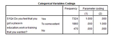
In the Categorical Variables Codings table below, you can see that our categorical variable, s1q4, has been recoded into dummy variables. No is again the baseline variable, just as it was in the simple logistic regression we ran with s1q4 in the previous section. We can tell because it has not been assigned a Parameter code. This is because as the baseline, comparison variable, it won’t be included in the logistic regression model. We will need this information when we want to analyse the odds ratios.
Block 0
Again, we’ve left out the output tables for Block 0, the predictions for the logistic model excluding our two independent variables. They won’t be very informative for us. However, if you’re interested in Block 0 output, please refer to the Simple Logistic Regression – One Continuous Variable section.
Block 1: Method = Enter
Remember that the Omibus Tests of Model Coefficients output table shows the results of a chi-square test to determine whether or not placement satisfaction has a statistically significant relationship with enrolment in full time education. The chi-square has produced a p-value of .000, making our placement satisfaction model significant at the 5% level.
We use the Cox & Snell r2 statistic calculated in the Model Summary output table below to gauge how much of the variation in full time enrolment is explained by this model. In this example, the r2 is low at 0.192. This shows that 19.2% of the variation in enrolment in full time education is explained by Sweep 1 placement satisfaction and total GCSE score in Year 11. This suggests despite our inclusion of two independent variables in this model, other factors are affecting a respondent’s enrolment in full time education.
In the Variables in the Equation table, we can see that the p-values for s1gcseptsnew and both of the dummy variables in s1q4 are 0.000, meaning that both the variables we’ve included in this model have statistically significant influence on respondent enrolment in full time education.
Does this final model have a better fit than the previous two logistic regression models we created? Looking at the output in the Model Summary table, we can see that the Cox & Snell r2 has risen from 0.168, its value in the simple logistic regression exploring s2q10 and s1gcseptsnew, to 0.192 in this multiple logistic regression. This means that 19.2% of the variation in enrolment in full time education can be explained by this model. Therefore, this model has a better fit than our previous two simple logistic regression models.
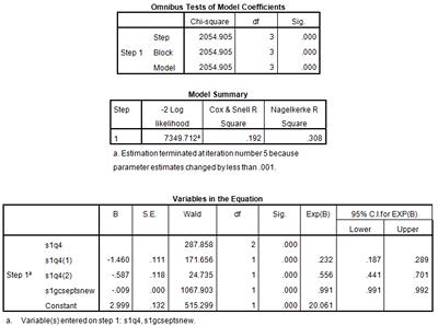
Examining the Block 1 output, we can see what (if anything) has changed in the predicted odds of being satisfied with Sweep 1 placement and being enrolled in full time education, now that the model controls for GCSE score. Remember that in this model, “No” was selected as our baseline comparison dummy variable and is called s1q4 in our model outputs. Because s1q4(1) (with a p-value of 0.000) is a significant predictor of the odds of enrolment in full time education, we can use the odds ratio information provided for us in the Exp(B) column to say that a respondent who was happy with her placement in Sweep 1 has odds of not being enrolled in full time education that are 0.232 the odds of someone who was unhappy with their placement. This means that again, those happy with their placements are more likely than those who were unhappy to be enrolled in full time education. We can compare that result to 0.097, the odds ratio for a satisfied respondent not being enrolled in full time education we calculated in the previous logistic regression. Again, an odds ratio less than 1 means that the odds of an event occurring are lower in that category than the odds of the event occurring in the baseline comparison variable. An odds ratio more than 1 means that the odds of an event occurring are higher in that category than the odds of the event occurring in the baseline comparison variable. So, yet again, even controlling for the influence of GCSE score (by including it in the logistic regression model), we’ve determined that students who were satisfied with their work, education, or training in Sweep 1 are more likely to be enrolled in full time education after secondary school than are students who were not satisfied with their placements in Sweep 1.
Summary
Here, you’ve run a multiple logistic regression using s2q10 as a binary categorical dependent variable and both s1q4 and s1gcseptsnew as independent variables. Using the output of this multiple logistic regression, you predicted the odds of a survey respondent being satisfied with their Sweep 1 placement and not being enrolled in full time education, much like you did in the previous logistic regression including only s2q10 and s1q4. You were able to determine how these predicted odds changed after you added s1gcseptsnew to the model and controlled for the influence of respondent GCSE score.