What are the odds that young people satisfied with their placements in Sweep 1 of the YCS will be enrolled in full time education in Sweep 2?
We’ve just run a simple logistic regression using s2q10 as a binary categorical dependent variable and s1gcseptsnew as a continuous independent variable. Suppose now we were interested to see if a respondent’s satisfaction with their education or work placements in Sweep 1 had any bearing on their enrolment in full time education in Sweep 2.
In order to answer the above question, we are going to fit a logistic regression model using s2q10 as our dependent variable and s1q4, respondent placement satisfaction, as our independent variable to see if we can find a significant relationship between these two variables.
Before we begin, we should run a frequency test on s1q4, to make sure that it is ready to be used in our analyses. Select Analyze, Descriptive Statistics, and then Frequencies. Find s1q4 in the variable list on the left and move it to the text box on the right. Click OK.
Notice in your output table that along with “Yes,” “To some extent,” and “No,” there is also a category called “Not answered,” which contains 90 cases in which there was no answer provided for the question s1q4. This is missing information and we don’t need to include it in our analyses. We should tell SPSS that the data in this category is missing data, so that it’s excluded from the tests we run using s1q4.
Luckily, this is very easy to do.
In Variable View, click to highlight any cell in the Name column on the far left side of the screen. Use Ctrl + F to pull up the Find and Replace dialogue box. This command will find variables in the dataset for you, which is really helpful when you are working in large datasets. Enter s1q4 in the text bar and select Find Next. The s1q4 cell should now to highlighted.
We know that we want to tell SPSS that the information in “Not answered” is missing data, but we don’t know what numerical value this category has been given in the dataset. We’ll need to know before we code the category as missing data. Follow the s1q4 row until you find the Values column. Click to open the Values cell in the s1q4 row.
You should now see that “Not answered” is coded as “-9.00” and that there are two more categories of unanswered questions/inapplicable data, given the values “4.00” and “5.00.” We’ll code these three categories as Missing.
To do this, simply move one cell to the right in the s1q4 row. This is the Missing column. Click to open this cell and select Discrete missing values. Enter “-9.00,” “4.00,” and “5.00” into the three text boxes provided. Click OK.
You should now see these missing values in the Missing cell of the s1q4 row. You’ve successfully coded these categories as containing missing data!
Now that s1q4 is ready to use, let’s run some exploratory analysis to determine if a relationship between these variables exists. If no relationship exists, there’s no need to continue on to our logistic regression.
If our independent variable was continuous, we would use a t test to compare means. However, in this section, our independent variable s1q4 is categorical, so we’ll start by running cross tabulations. Select Analyze, Descriptive Statistics, and Crosstabs. Move s2q10 into the Column(s) box and s1q4 into the Row(s) box. Click the Statistics button and select Chi-Square. Click Continue. Because we are curious about s1q4, we’d also like to see some row percentages. Click on Cells, and then under the Percentages header, select Row. Click Continue. Then, click OK to run the crosstabulation.
Your output should look like the tables on the right.
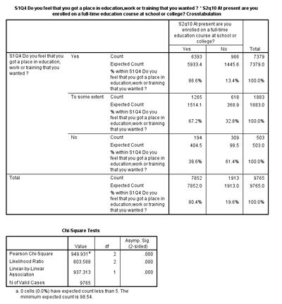
Is there a significant relationship between s2q10 and s1q4? How can you tell?
Now we can fit our logistic regression model using s2q10 as the dependent variable and s1q4 as the independent variable.
Select Analyze, Regression, and then Binary Logistic.
Move s2q10 to the Dependent text box. Move s1q4 to the Covariates text box. Because s1q4 is a categorical variable, we have to tell SPSS to create dummy variables for each of the categories. (SPSS will do this for us in logistic regression – unlike in linear regression, when we had to create the dummies ourselves.) To tell SPSS that s1q4 is a categorical variable, click Categorical in the upper right corner of the Logistic Regression text box.
Move s1q4 from the Covariates text box on the left to the Categorical Covariates text box on the right. Click Continue.
The original Logistic Regression dialogue box should now have s1q4(Cat) in the Covariates text box.
We can also have SPSS calculate confidence intervals for s1q4 for us. In the Logistic Regression dialogue box you should have open, click Options. Under Statistics and Plots, select CI for exp(B). This should already be set at 95%.
Click Continue and then OK in the original Logistic Regression dialogue box.
Now we can examine the output.
You can see in the Case Processing Summary that again, there are around 4,000 cases listed as Missing and therefore not included in the analysis.
In the Dependent Variable Encoding table, you can see that enrolment in full time education (“Yes”) is coded as 0 and not being enrolled in full time education (“No”) is coded as 1. Just as in our previous logistic regression model, investigating s2q10 and GCSE score, we will be predicting the odds of not being enrolled in full time education.
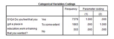
The Categorical Variables Codings table shows us the frequencies of respondent satisfaction with their placement in education, work, or training. In addition, it also tells us that the three categories of s1q4 have been recoded in our logistic regression as dummy variables. In logistic regression, just as in linear regression, we are comparing groups to each other. In order to make a comparison, one group has to be omitted from the comparison to serve as the baseline. In our logistic regression, “No” has been selected as the baseline (or constant) dummy variable to which we will compare the predictions for “Yes” and “To some extent.” Therefore, “No” won’t be included in our model. (You can see that in the table below it isn’t coded with a “1” in any case, because it is the baseline, comparison category and has not been added to the model. You can change the category to be used as the baseline to either the first or last categories – this is done where you specify that the variable is categorical under the Categorical button in the Logistic Regression dialogue box.
Block 0
As we’re not going to use any of the information provided for us in Block 0, the output has been left out of this worksheet. If you’d like to work through some of the information provided for you in Block 0, you can use the interpretation provided above for the s2q10 and s1gcseptsnew logistic regression model we did on the previous page.
Block 1: Method = Enter
Remember that the Omibus Tests of Model Coefficients output table shows the results of a chi-square test to determine whether or not placement satisfaction has a statistically significant relationship with enrolment in full time education. The chi-square has produced a p-value of 0.000, making our placement satisfaction model significant at the 5% level.
We use the Cox & Snell r2 statistic calculated in the Model Summary output table below to gauge how much of the variation in full time enrolment is explained by this model. In this example, the r2 is low at 0.079. This shows that only 7.9% of the variation in enrolment in full time education is explained by Sweep 1 placement satisfaction. This suggests that other factors are affecting a respondent’s enrolment in full time education.
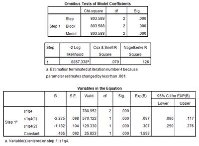
Take a look at the Variables in the Equation output table above. Let’s first look at the significance levels. S1q4(1), or “Yes,” has a p-value of 0.000, making it significant at the p < .05 level. S1q4(2), or “To some extent,” on the other hand, has a p-value of 0.000, telling us that it is also a significant predictor of full time enrolment in education.
Remember that in this model, “No” was selected as our baseline comparison dummy variable and is called s1q4 in our model outputs. Because s1q4(1) (“Yes, I feel I got a place I wanted”) has a p-value of 0.000 and is a significant predictor of the odds of enrolment in full time education, we can use the odds ratio information provided for us in the Exp(B) column to say that a respondent who was happy with her placement in Sweep 1 has odds of not being enrolled in full time education that are 0.097 the odds of someone who was unhappy with their placement. This means that those happy with their placements are more likely than those who were unhappy to be enrolled in full time education. An odds ratio less than 1 means that the odds of an event occurring are lower in that category than the odds of the event occurring in the baseline comparison variable. An odds ratio more than 1 means that the odds of an event occurring are higher in that category than the odds of the event occurring in the baseline comparison variable.
A respondent who was satisfied “to some extent” with their placement in work, education, or training [s1q4(2)] has odds of not being enrolled in full time education that are _____________ of the odds of a respondent who was not satisfied with their placement. This means that those who were only partially satisfied with their placement are ________ likely than those who were not satisfied to be enrolled in full time education.
In addition, SPSS has calculated confidence intervals for us. Remember that confidence intervals allow us to extend out analyses from the sample in our data to the population as a whole. We can say, with 95% confidence, that for the entire population of England, young people who were satisfied with their placements in Sweep 1 have odds of not being enrolled in full time education that are 0.080 to 0.117 the odds of people who were not satisfied with their placements in Sweep 1.
Summary
First, you used a chi square test test to determine whether or not a statistically significant relationship existed between our categorical independent variable s1q4 and our categorical dependent variable s2q10. Then, using simple logistic regression, you predicted the odds of a survey respondent not being enrolled in full time education with regard to their satisfaction with their placement in work or education in Sweep 1. Finally, using the odds ratios provided by SPSS in the Exp(B) column of the Variables in the Equation output table, you were able to interpret the odds of students satisfied with their placements not being enrolled in full time education in Sweep 2.
Note: as we are making changes to a dataset we’ll continue using for the rest of this section, please make sure to save your changes before you close down SPSS. This will save you having to repeat sections you’ve already completed.