Simple Logistic Regression: One Continuous Independent Variable

What are the odds that young people with high GCSE scores in Sweep 1 of the YCS will be enrolled in full time education in Sweep 2?

Our variable of interest, enrolment in full time education, has two categories. As a result, we can model it using logistic regression, which requires a binary variable as the outcome. First, we can fit a logistic regression model with s2q10 as the dependent variable and s1gcseptsnew as the independent variable. However, before we begin, we should run exploratory bivariate analysis to get some answers about the relationship between s1gcseptsnew and s2q10.

Because s1gcseptsnew is a continuous variable, we can run a two-sample t test to determine if there is a statistically significant difference in the mean GCSE scores for those who enrolled in education full time after secondary school and those who did not. This, like all exploratory analysis, can help us determine whether or not it is worth fitting a logistic regression model for these variables. If the difference in mean GCSE score with respect to s2q10 is insignificant, running a logistic regression wouldn’t be the best use of our time, as our results wouldn’t be significant.

In addition to telling us if we’re on the right track with our analysis, running this simple t test will also provide us with the frequencies of those who answered “Yes” and those who answered “No,” which will allow us to calculate the percentage of the survey respondents who were enrolled and those who were not enrolled in full time education.

Go to Analyze, Compare Means, and then Independent-Samples T Test.

Move s1gcseptsnew into the Test Variables(s) box and s2q10 into the Grouping Variable box.

Click on Define Groups and enter 1 in the Group 1 box and 2 in the Group 2 box, because 1=Yes and 2=No in s2q10 in our dataset. (You can check this by using Ctrl + F to find s2q10 in the variable list in Variable View and clicking to open the Values cell in the s2q10 row. This will show you what values have been given to each of the categories in s2q10).
Click Continue. Click OK to close the Independent-Samples T Test dialogue box.

Your output should look like the table on the right.

You can use the information in the t test output tables to answer the following questions:

What is the mean GCSE score for respondents who were enrolled in full time education?

What is the mean GCSE score for respondents who were not enrolled in full time education?

Take a look at the significance levels in the Independent Sample Test output box. Is there a significant difference between the mean GCSE scores for s2q10 respondents who were enrolled in full time education and those who were not?

Because we’ve just discovered that there is a significance difference between mean respondent GCSE scores, we know that there is a relationship between s2q10 and s1gcseptsnew. We can now continue on to fitting a logistic regression model to further explore this relationship.

Select Analyze, Regression, and then Binary Logistic.

Find our variable s2q10 from the variable list on the left of the dialogue box and move it the Dependent text box. Find the variable s1gcseptsnew and move it to the Covariates text box. Click OK.

You will now have several output tables open in the Output Viewer. Let’s take a look at them.

The first table, called the Case Processing Summary, shows us that 9,705 cases were included in this logistic regression, and 4,298 are coded as Missing.

In our dataset, in the variable s2q10, “Yes” is coded as “1” and “No” is coded as “2.” An answer of “No,” therefore, has been arbitrarily given a larger numeric code (as 2 is greater than 1). In logistic regression in SPSS, the variable category coded with the larger number (in this case, “No”) becomes the event for which our regression will predict odds. In other words, because the outcome “No” is coded as “2” in the dataset, the logistic regression will predict the odds of a respondent answering “No” to the question of whether or not they were enrolled in full time education. Because we are now predicting the odds of a respondent answering “No,” this answer becomes the success in our model, or “1.” An answer of “Yes” is a failure, or “0.” The Dependent Variable Encoding table shows you that the Original Values of “Yes” and “No” (the answers to s2q10) are coded as “0” and “1” in this analysis.

As you can see in your Output window, SPSS gives you many, many tables, most of which you won’t need to worry about. Here, we’ll highlight just the main points. The other tables become more useful as you do more in-depth analysis – we don’t have to worry about them now.

The output tables in Block 0: Beginning Block show the full time education enrolment predictions before the addition of our independent variable s1gcseptsnew into the model. Block 0 shows us the odds of a respondent not being enrolled in full time education without the influence of GCSE score.

Block 0: Beginning Block

In the Variables in the Equation table, we can see the odds of not being enrolled in full time education. These odds ratios are presented as the Exp(B) output in this table. Here we see that without the addition of GCSE score, the odds that a respondent would not be enrolled in full time education are 0.237 the odds that a respondent would be enrolled in full time education.

 

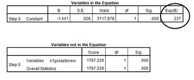
In the Variables not in the Equation table, we see the predicted significance for the variable s1gcseptsnew. If p < 0.05, this table predicts GCSE score will be significant and that the addition of the second variable will improve the fit of the model. Before we move on to the logistic regression that includes s1gcseptsnew, take a look at the information provided for us here.

We can see that the predicted p-value for the s1gcseptsnew in this model is 0.000.

What do you think the addition of our explanatory variable will do to our model? Will it improve the fit of this logistic regression? Will we be better able to predict odds when we add s1gcseptsnew to our model? Why or why not?

Let’s move on to Block 1: Method = Enter, and see what changes (if any) our independent variable has on the predicted odds of a respondent not being enrolled in full time education.

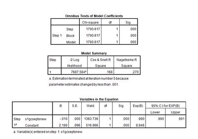
Block 1: Method = Enter

The Omnibus Tests of Model Coefficients table shows us the results of a chi-square test. This hypothesis test examines whether or not there is a statistically significant impact of GCSE score on the prediction of full time enrolment in education after secondary school. In order to accept that GCSE score has statistically significant influence on full time enrolment in education, the p-value must be less than 0.05.

Based on the results above, do you think GCSE score has a statistically significant impact on the prediction of full time education enrolment?

We use the Cox & Snell r² statistic calculated in the Model Summary output table below to gauge how much of the variation in full time enrolment in education is explained by this model, and therefore how well our model fits our data. In this example, the r² is 0.168. This shows that 16.8% of the variation in educational enrolment is explained by GCSE score (as 0.168 X 100 = 16.8). This indicates that other factors are affecting a respondent’s enrolment in full time education.

Is our logistic regression model a good one? How can you tell?

In the Variables in the Equation table, we can see that the p-value for s1gcseptsnew in this regression is p=0.000, meaning this variable does have a statistically significant influence on respondent enrolment in full time education.

As you can see, actually running the logistic regression is not a problem – as long as you remember to put the binary outcome variable in the correct box in SPSS, it is difficult to go wrong! However, the interpretation of the results is a bit trickier – and the interpretation is what you are really interested in.

As noted above, we can easily see that the relationship between the GCSE score of the respondent and enrolment in full time is significant (as shown by the p-value being less than 0.05). But what is this relationship? For every one point increase in GCSE score, the log-odds of someone not being enrolled in full time education decreases by 0.010 units. This does not mean much in terms of interpretation, which is unfortunate, because logistic regression actually conducts the analysis on the log odds. A better way of interpreting this is by using the odds ratio – which is included in the Exp(B) column, the final column of the table. In our example here, the odds ratio is 0.990. Because s1gcseptsnew is a continuous variable, we can say that with every point increase in GCSE score, the odds of not being enrolled in full time education after secondary school are multiplied by 0.990. Because 0.990 is less than 1, any odds being multiplied by 0.990 will decrease. Therefore, as GCSE score increases, the odds of not being enrolled in full time education decrease. Young people with higher GCSE scores are more likely to be enrolled in full time education after secondary school.

Logistic regression results can also be interpreted as probabilities – but we will not do this here.

This difference by GCSE score is subtly reflected in the mean GCSE scores for s1gcseptsnew respondents we calculated before running this logistic regression. The mean GCSE score for respondents who answered “Yes” to full time enrolment in education was 432.85. The mean GCSE score for respondents who answered “No” to full time enrolment in education was 290.70.

Summary

First, you used an independent-sample (or two-sample) t test to determine whether or not a statistically significant relationship existed between our continuous independent variable s1gcseptsnew and our categorical dependent variable s2q10. Then, using simple logistic regression, you predicted the odds of a survey respondent not being enrolled in full time education after secondary school with regard to their GCSE score. You’ve learned that the results of a logistic regression are presented first as log-odds, but that those results often cause problems in interpretation. While the results of a logistic regression model can also be interpreted as probability, a favoured way of describing the results is to use the odds ratio provided by SPSS in the Exp(B) column of the Variables in the Equation output table.

Note: as we are making changes to a dataset we’ll continue using for the rest of this section, please make sure to save your changes before you close down SPSS. This will save you having to repeat sections you’ve already completed.